MMM API Migration Guide#

This guide helps you migrate from the old MMM class (pymc_marketing.mmm.MMM) to the new multidimensional MMM class (pymc_marketing.mmm.multidimensional.MMM).

Why Migrate?#

The new MMM class provides several improvements:

Multidimensional Support: Native support for hierarchical and multidimensional models
Cleaner API: More explicit model building steps with better separation of concerns
Flexible Priors: Choose between total pooling (shared parameters) or channel-specific priors
Enhanced Plotting: Reorganized plotting API under mmm.plot.* namespace
Improved Budget Optimization: New wrapper class for more flexible optimization scenarios

This guide covers all API changes with side-by-side code comparisons to make your migration straightforward.

1. Import Path Change#

The primary import path has changed:

Old:

from pymc_marketing.mmm import MMM

New:

from pymc_marketing.mmm.multidimensional import MMM

The new class is imported from the multidimensional submodule during the migration. From version 0.20.0 onwards, the new class is imported from the root pymc_marketing.mmm.MMM module.

from pymc_marketing.mmm import MMM as MMM_old
from pymc_marketing.mmm import GeometricAdstock, LogisticSaturation
from pymc_marketing.mmm.multidimensional import MMM as MMM_new

2. Model Initialization & Model Config Defaults#

The new MMM class initializes is the same as the old one.

mmm_old = MMM_old(
    date_column="date_week",
    channel_columns=["x1", "x2"],
    adstock=GeometricAdstock(l_max=8),
    saturation=LogisticSaturation(),
)

mmm_old.model_config

{'intercept': Prior("Normal", mu=0, sigma=2, dims=()),
 'likelihood': Prior("Normal", sigma=Prior("HalfNormal", sigma=2, dims=()), dims="date"),
 'gamma_control': Prior("Normal", mu=0, sigma=2, dims="control"),
 'gamma_fourier': Prior("Laplace", mu=0, b=1, dims="fourier_mode"),
 'adstock_alpha': Prior("Beta", alpha=1, beta=3, dims="channel"),
 'saturation_lam': Prior("Gamma", alpha=3, beta=1, dims="channel"),
 'saturation_beta': Prior("HalfNormal", sigma=2, dims="channel")}

mmm_new = MMM_new(
    date_column="date_week",
    channel_columns=["x1", "x2"],
    adstock=GeometricAdstock(l_max=8),
    saturation=LogisticSaturation(),
)

mmm_new.model_config

{'intercept': Prior("Normal", mu=0, sigma=2, dims=()),
 'likelihood': Prior("Normal", sigma=Prior("HalfNormal", sigma=2, dims=()), dims="date"),
 'gamma_control': Prior("Normal", mu=0, sigma=2, dims="control"),
 'gamma_fourier': Prior("Laplace", mu=0, b=1, dims="fourier_mode"),
 'adstock_alpha': Prior("Beta", alpha=1, beta=3, dims="channel"),
 'saturation_lam': Prior("Gamma", alpha=3, beta=1, dims="channel"),
 'saturation_beta': Prior("HalfNormal", sigma=2, dims="channel")}

mmm_new.model_config == mmm_old.model_config

True

3. Adding Original Scale Variables to the Inference Data#

The new API allows you to store variable contribution in the original scale in the inference data attribute.

mmm = MMM(...)

# Step 1: Build the model explicitly
mmm.build_model(X_train, y_train)

# Step 2: Add original scale contribution variables (optional but recommended)
mmm.add_original_scale_contribution_variable(var=["channel_contribution", "y"])

# Step 3: Fit the model
mmm.fit(X_train, y_train)

Why `add_original_scale_contribution_variable()`?#

This method stores unscaled (original scale) contribution variables in idata["posterior"]. This is particularly useful when:

You want to analyze contributions in the original units (dollars, impressions, etc.)
You need to compare contributions across different scales

Without this call, you would need to manually reverse the scaling transformation during analysis.

4. Parameter Naming Changes#

Some internal parameter names have changed. Update your code if you access parameters directly:

Old Name	New Name
`intercept`	`intercept_contribution`

Example:

# Old
az.summary(mmm.fit_result, var_names=["intercept"])

# New
az.summary(mmm.fit_result, var_names=["intercept_contribution"])

5. Plotting API Changes#

New Access Pattern#

Plotting functions are now accessed through the plot attribute:

Old:

mmm.plot_prior_predictive(...)
mmm.plot_posterior_predictive(...)

New:

mmm.plot.prior_predictive(...)
mmm.plot.posterior_predictive(...)

Renamed Functions#

Several plotting functions have been renamed for clarity:

Old Function	New Function
`plot_components_contributions`	`plot.contributions_over_time`
`plot_direct_contribution_curves`	`plot.saturation_scatterplot`
`plot_channel_contribution_grid`	`plot.sensitivity_analysis`

Examples#

Contributions over time:

# Old
fig = mmm.plot_components_contributions(original_scale=True)

# New
fig = mmm.plot.contributions_over_time()

Saturation curves:

# Old
fig = mmm.plot_direct_contribution_curves()

# New
fig = mmm.plot.saturation_scatterplot()

Channel-Specific Parameter Plots#

For channel-specific parameters, use ArviZ directly:

import arviz as az

# Plot posterior for channel-specific parameters
az.plot_posterior(
    mmm.fit_result,
    var_names=["adstock_alpha", "saturation_lam"],
    coords={"channel": mmm.channel_columns}
)

6. Sensitivity Analysis Workflow#

Sensitivity analysis now follows a two-step process, separating computation from visualization.

Old Approach (Single Function)#

# Old - computation and plotting combined
fig = mmm.plot_channel_contribution_grid(start=0, stop=1.5, num=12)

New Approach (Two Steps)#

import numpy as np

# Step 1: Run the sensitivity sweep (stores results in idata)
mmm.sensitivity.run_sweep(
    sweep_values=np.linspace(0, 1.5, 12),
    var_name="channel_contribution",
)

# Step 2: Visualize the results
fig = mmm.plot.sensitivity_analysis()

Benefits of the New Approach#

Reusable Results: Sweep results are stored in idata["sensitivity_analysis"] and can be accessed later
Flexible Visualization: Plot the same results in different ways without re-running the sweep
Custom Analysis: Access raw sweep results for custom analysis:

# Access sensitivity results directly
sensitivity_data = mmm.idata["sensitivity_analysis"]

7. Budget Optimization Changes#

Budget optimization now uses a dedicated wrapper class for more flexibility.

Old Approach#

# Old - direct method on MMM
allocation, result = mmm.optimize_budget(
    budget=1000,
    num_days=30,
    budget_bounds={"x1": [0, 500], "x2": [0, 500]},
)

New Approach#

import xarray as xr
from pymc_marketing.mmm.multidimensional import MultiDimensionalBudgetOptimizerWrapper

# Step 1: Create the optimizer wrapper with date range
optimizable_model = MultiDimensionalBudgetOptimizerWrapper(
    model=mmm,
    start_date="2023-01-01",
    end_date="2023-12-31",
)

# Step 2: Define budget bounds as xarray DataArray
budget_bounds = xr.DataArray(
    data=[[0, 500], [0, 500]],
    dims=["channel", "bound"],
    coords={
        "channel": ["x1", "x2"],
        "bound": ["lower", "upper"],
    },
)

# Step 3: Run optimization
allocation, result = optimizable_model.optimize_budget(
    budget=1000,
    budget_bounds=budget_bounds,
)

# Step 4: Visualize results
fig = optimizable_model.plot.budget_allocation()

Key Differences#

Aspect	Old	New
Budget bounds	Dictionary	`xarray.DataArray`
Date range	`num_days` parameter	`start_date`/`end_date` in wrapper
Plotting	`mmm.plot_budget_allocation()`	`optimizable_model.plot.budget_allocation()`

Benefits of the New Approach#

Time-Aware Optimization: Specify exact date ranges for optimization
Multidimensional Bounds: Use xarray for complex constraint structures (e.g., time-varying bounds)
Separation of Concerns: Optimization logic is separate from the core model

8. Complete Example#

Here’s a minimal end-to-end example using the new API:

import arviz as az
import matplotlib.pyplot as plt
import numpy as np
import pandas as pd

from pymc_marketing.mmm.components.adstock import GeometricAdstock
from pymc_marketing.mmm.components.saturation import LogisticSaturation
from pymc_marketing.mmm.multidimensional import MMM

az.style.use("arviz-darkgrid")
plt.rcParams["figure.figsize"] = [12, 7]
plt.rcParams["figure.dpi"] = 100

seed: int = sum(map(ord, "mmm"))
rng: np.random.Generator = np.random.default_rng(seed=seed)

%load_ext autoreload
%autoreload 2
%config InlineBackend.figure_format = "retina"

# Load sample data
data_url = "https://raw.githubusercontent.com/pymc-labs/pymc-marketing/main/data/mmm_example.csv"
data = pd.read_csv(data_url, parse_dates=["date_week"])

# Define channel columns
channel_columns = ["x1", "x2"]

# Create the model (new API)
mmm = MMM(
    date_column="date_week",
    channel_columns=channel_columns,
    adstock=GeometricAdstock(l_max=8),
    saturation=LogisticSaturation(),
)

# Prepare data
X = data[["date_week", *channel_columns]]
y = data["y"]

# Build model explicitly (new step)
mmm.build_model(X, y)

# Add original scale contribution variables (recommended)
mmm.add_original_scale_contribution_variable(var=["channel_contribution", "y"])

# Fit the model
mmm.fit(X, y, chains=4, draws=1_000, target_accept=0.9, random_seed=rng)
mmm.sample_posterior_predictive(X, random_seed=rng)


# Analyze results using the new plotting API
mmm.plot.posterior_predictive()
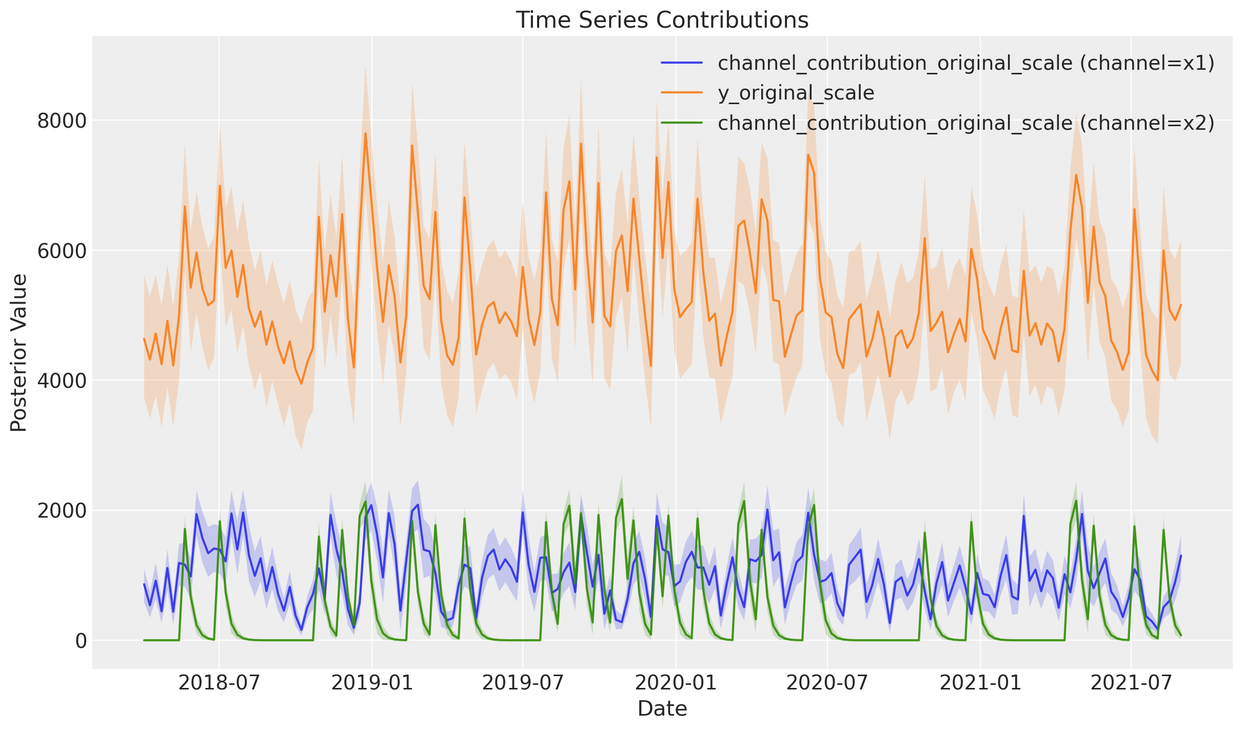
mmm.plot.contributions_over_time(
    var=["channel_contribution_original_scale", "y_original_scale"],
    combine_dims=True,
    figsize=(12, 7),
)

../../_images/90c160e4bb575c55e8aa950eca83a35c83222bfc56d44a229c7be6e99a58fb97.png

10. Quick Reference Summary#

Import Changes#

Old	New
`from pymc_marketing.mmm import MMM`	`from pymc_marketing.mmm.multidimensional import MMM`

Model Building#

Old	New
Implicit (during `fit()`)	Explicit: `build_model()` then `add_original_scale_contribution_variable()`

Prior Defaults#

Behavior	Old	New
Default	Channel-specific (`dims="channel"`)	Total pooling (shared)
Channel-specific	Implicit	Add `dims="channel"` to `model_config`

Parameter Names#

Old	New
`intercept`	`intercept_contribution`

Plotting API#

Old	New
`mmm.plot_*()`	`mmm.plot.*()`
`plot_components_contributions`	`plot.contributions_over_time`
`plot_direct_contribution_curves`	`plot.saturation_scatterplot`
`plot_channel_contribution_grid`	`plot.sensitivity_analysis`

Sensitivity Analysis#

Old	New
`mmm.plot_channel_contribution_grid(...)`	`mmm.sensitivity.run_sweep(...)` then `mmm.plot.sensitivity_analysis()`

Budget Optimization#

Old	New
`mmm.optimize_budget(...)`	`MultiDimensionalBudgetOptimizerWrapper(model=mmm, ...).optimize_budget(...)`
`budget_bounds` as dict	`budget_bounds` as `xarray.DataArray`
`num_days` parameter	`start_date`/`end_date` in wrapper constructor

%load_ext watermark
%watermark -n -u -v -iv -w

Last updated: Tue, 17 Feb 2026

Python implementation: CPython
Python version       : 3.13.11
IPython version      : 9.9.0

arviz         : 0.23.1
matplotlib    : 3.10.8
numpy         : 2.3.5
pandas        : 2.3.3
pymc_extras   : 0.6.1.dev9+g828353dcd
pymc_marketing: 0.17.1

Watermark: 2.6.0

MMM API Migration Guide#

Why Migrate?#

1. Import Path Change#

2. Model Initialization & Model Config Defaults#

3. Adding Original Scale Variables to the Inference Data#

Why add_original_scale_contribution_variable()?#

4. Parameter Naming Changes#

5. Plotting API Changes#

New Access Pattern#

Renamed Functions#

Examples#

Channel-Specific Parameter Plots#

6. Sensitivity Analysis Workflow#

Old Approach (Single Function)#

New Approach (Two Steps)#

Benefits of the New Approach#

7. Budget Optimization Changes#

Old Approach#

New Approach#

Key Differences#

Benefits of the New Approach#

8. Complete Example#

10. Quick Reference Summary#

Import Changes#

Model Building#

Prior Defaults#

Parameter Names#

Plotting API#

Sensitivity Analysis#

Budget Optimization#

Why `add_original_scale_contribution_variable()`?#